Output
By default, metrics are printed to standard output using print_metric(). You can provide your own
metric recording funtion. It should take three arguments: count of items,
elapsed time in seconds, and name, which can be None:
>>> def my_metric(name, count, elapsed):
...     print("Iterable %s produced %d items in %d milliseconds"%(name, count, int(round(elapsed*1000))))
...
>>> _ = instrument.all(math_is_hard(5), metric=my_metric, name="bogomips")
>>> list(_)
Iterable bogomips produced 5 items in 5000 milliseconds
[0, 1, 4, 9, 16]
Unless individually specified, metrics are reported using the global
instrument.default_metric(). To change the active default, simply assign another
metric function to this attribute. In general, you should configure your
metric functions at program startup, before recording any metrics.
make_multi_metric() composes several metrics functions together, for simultaneous
display to multiple outputs.
Loggging
logging writes metrics to a standard library logger, using the metric’s name.
>>> from instrument.output.logging import log_metric
>>> _ = instrument.all(math_is_hard(5), metric=log_metric, name="bogomips")
>>> list(_)
INFO:instrument.bogomips:5 items in 5.00 seconds
[0, 1, 4, 9, 16]
Comma Separated
csv saves raw metrics as comma separated text files.
This is useful for conducting external analysis. csv is threadsafe; use
under multiprocessing requires some care.
CSVFileMetric saves all metrics to a single file with three
columns: metric name, item count & elapsed time. Create an instance of this
class and pass its CSVFileMetric.metric() method to measurement
functions. The outfile parameter controls where to write data; an existing
file will be overwritten.
>>> import tempfile, os.path
>>> csv_filename = os.path.join(tempfile.gettempdir(), "my_metrics_file.csv")
>>> from instrument.output.csv import CSVFileMetric
>>> csvfm = CSVFileMetric(csv_filename)
>>> _ = instrument.all(math_is_hard(5), metric=csvfm.metric, name="bogomips")
>>> list(_)
[0, 1, 4, 9, 16]
CSVDirMetric saves metrics to multiple files, named after each
metric, with two columns: item count & elapsed time. This class is global to
your program; do not manually create instances. Instead, use the classmethod
CSVDirMetric.metric(). Set the class variable outdir to a directory
in which to store files. The contents of this directory will be deleted on
startup.
Both classes support at dump_atexit flag, which will register a handler to
write data when the interpreter finishes execution. Set to false to manage
yourself.
Summary Reports
table reports aggregate statistics and plot generates plots (graphs). These are
useful for benchmarking or batch jobs; for live systems, statsd is a better choice.
table and plot are threadsafe; use under multiprocessing requires some care.
TableMetric and PlotMetric are global to your program; do not manually create
instances. Instead, use the classmethod metric(). The dump_atexit flag will register a
handler to write data when the interpreter finishes execution. Set to false to manage yourself.
Tables
TableMetric prints pretty tables of aggregate population statistics. Set the class variable outfile to a file-like object (defaults to stderr):
>>> from instrument.output.table import TableMetric
>>> _ = instrument.all(math_is_hard(5), metric=TableMetric.metric, name="bogomips")
>>> list(_)
[0, 1, 4, 9, 16]
You’ll get a nice table for output:
Name           Count Mean        Count Stddev        Elapsed Mean        Elapsed Stddev
alice            47.96              28.44               310.85               291.16
bob              50.08              28.84               333.98               297.11
charles          51.79              29.22               353.58               300.82
Plots
PlotMetric generates plots using matplotlib. Plots are saved to
multiple files, named after each metric. Set the class variable outdir to a
directory in which to store files. The contents of this directory will be
deleted on startup.
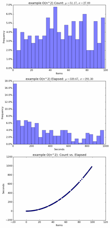
Sample plot for an O(n2) algorithm
statsd
For monitoring production systems, the statsd_metric() function can be used to record
metrics to statsd and
graphite. Each metric will generate two buckets: a count
and a timing.